Getting started#
This page shows how to install ternary-diagram, draw and save your first ternary diagram, pass compositions in the order of the vertices, place diagrams on existing axes, and control how chemical formulas in labels are formatted.
At the end, a table lists every drawing method and the page that explains it in detail.
Installation#
Install the package from PyPI with pip:
pip install ternary-diagram
or from conda-forge with conda:
conda install -c conda-forge ternary-diagram
The only runtime dependencies are numpy and matplotlib.
Your first diagram#
Create a matplotlib figure, pass its axes to TernaryDiagram together with the names of the three components, and draw on the diagram with its methods.
Here, scatter() plots randomly generated compositions as points and plot() draws a line between two compositions.
Because the diagram is an ordinary matplotlib figure, fig.savefig saves it to an image file.
import matplotlib.pyplot as plt
import numpy as np

from ternary_diagram import TernaryDiagram
rng = np.random.default_rng(0)
compositions = rng.dirichlet([2, 2, 2], size=30)

fig, ax = plt.subplots(layout="constrained")
td = TernaryDiagram(["Li2O", "La2O3", "TiO2"], ax=ax)
points = td.scatter(compositions)
lines = td.plot([[0.6, 0.2, 0.2], [0.1, 0.3, 0.6]], color="gray")
fig.savefig("my_diagram.png", dpi=300)
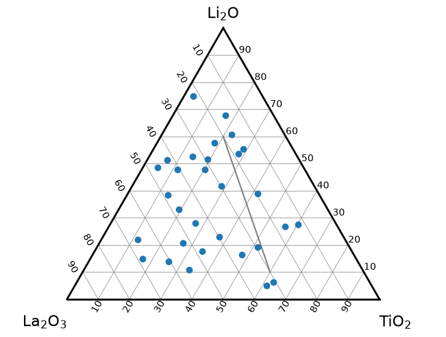
The methods return the matplotlib objects they create (here a PathCollection and a list of Line2D), and keyword arguments such as color are passed to matplotlib as they are.
Passing compositions#
Compositions are given as an array-like of shape (n, 3): one row per point and one column per component.
The columns are in the same order as the names passed to TernaryDiagram, and the names are placed at the vertices in the order top, bottom left, bottom right.
So the first column is the fraction of the top component, the second column is the bottom-left component and the third column is the bottom-right component.
The rows do not have to sum to 1, because each row is normalized before it is plotted.
In the next example, [0.5, 0.25, 0.25] and [2, 1, 1] describe the same ratio and are drawn at the same point.
fig, ax = plt.subplots(layout="constrained")
td = TernaryDiagram(["A", "B", "C"], ax=ax)
fractions = td.scatter([[0.5, 0.25, 0.25]], s=200, label="[0.5, 0.25, 0.25]")
ratios = td.scatter([[2, 1, 1]], marker="x", s=60, c="black", label="[2, 1, 1]")
legend = ax.legend(loc="upper left")
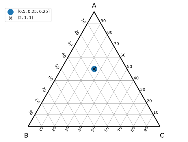
The two points have the same position on the axes:
print(np.allclose(fractions.get_offsets(), ratios.get_offsets()))
True
Tabular data can be passed as it is.
A pandas DataFrame with three columns, a two-dimensional numpy array or a list of lists is accepted wherever a composition is expected.
Select the columns in the order of the vertices, for example td.scatter(df[["Li2O", "La2O3", "TiO2"]]) for a DataFrame df that has more columns.
Drawing on existing axes#
TernaryDiagram draws on the axes given by ax, so a ternary diagram can go into any figure you have already created; without ax, it draws on the current axes (plt.gca()).
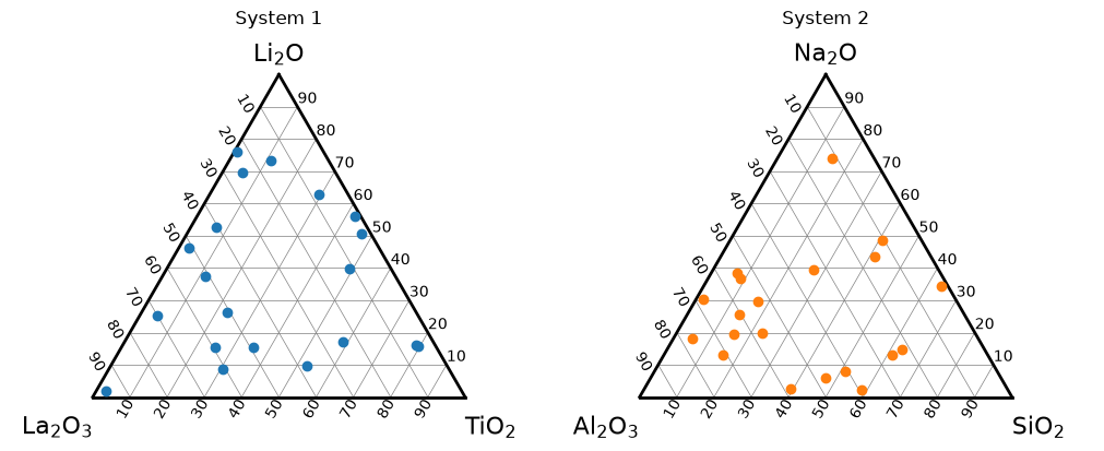
To place several diagrams side by side, create the panels with plt.subplots and pass one axes to each TernaryDiagram.
Each diagram keeps its own components, data and settings.
rng = np.random.default_rng(1)

fig, axes = plt.subplots(1, 2, figsize=(10, 4), layout="constrained")

left = TernaryDiagram(["Li2O", "La2O3", "TiO2"], ax=axes[0])
left_points = left.scatter(rng.dirichlet([1, 1, 1], size=20))
left_title = axes[0].set_title("System 1", pad=24)

right = TernaryDiagram(["Na2O", "Al2O3", "SiO2"], ax=axes[1])
right_points = right.scatter(rng.dirichlet([1, 1, 1], size=20), color="tab:orange")
right_title = axes[1].set_title("System 2", pad=24)
The page Layout and colorbars explains how the diagrams work with matplotlib’s layout engines, including subfigures.
Chemical formula labels#
By default, the vertex labels are treated as chemical formulas and their numbers are written as subscripts: Li2O is shown as Li$_{2}$O in matplotlib’s math text.
Pass auto_latex_notation=False to TernaryDiagram to show the labels exactly as you typed them.
fig, axes = plt.subplots(1, 2, figsize=(10, 4), layout="constrained")
formatted = TernaryDiagram(["Li2O", "La2O3", "TiO2"], ax=axes[0])
as_typed = TernaryDiagram(
    ["Li2O", "La2O3", "TiO2"], ax=axes[1], auto_latex_notation=False
)
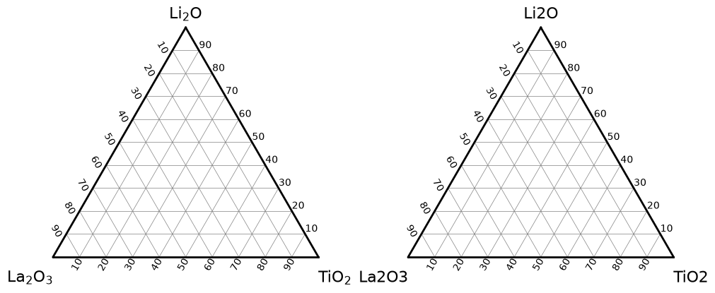
The texts of the vertex labels show the difference:
print([label.get_text() for label in formatted.vertex_labels_])
print([label.get_text() for label in as_typed.vertex_labels_])
['Li$_{2}$O', 'La$_{2}$O$_{3}$', 'TiO$_{2}$']
['Li2O', 'La2O3', 'TiO2']
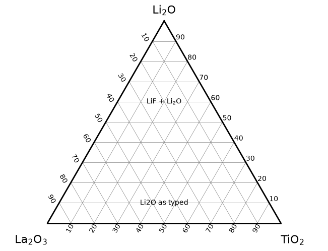
The setting chosen when the diagram is created also applies to text(), which places a label centered exactly at a composition.
With auto_latex_notation=None (the default), text follows the setting of the diagram, and True or False overrides it for one call.
text formats only the words, separated by spaces, that look like chemical formulas, so "LiF + Li2O" becomes "LiF + Li$_{2}$O".
fig, ax = plt.subplots(layout="constrained")
td = TernaryDiagram(["Li2O", "La2O3", "TiO2"], ax=ax)
inherited = td.text("LiF + Li2O", [0.6, 0.2, 0.2])
overridden = td.text("Li2O as typed", [0.1, 0.45, 0.45], auto_latex_notation=False)
Annotations follow their own rule, which you choose with the auto_latex_notation argument of annotate() and of scatter (for the labels given by annotations):
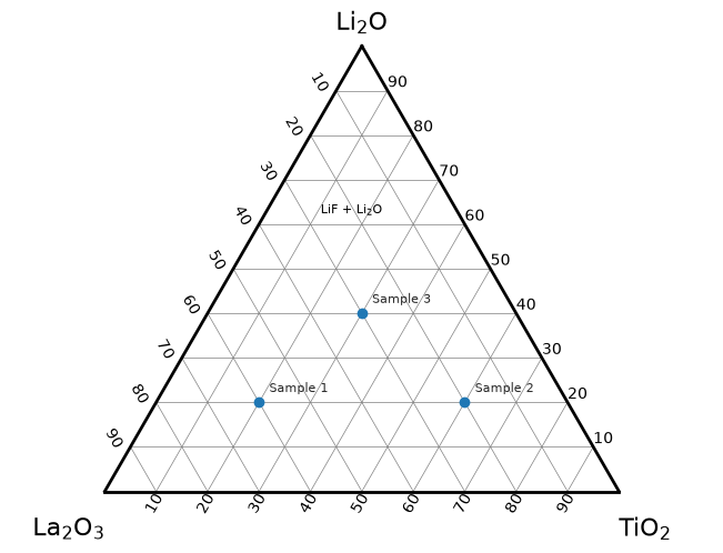
Trueformats only the words that look like chemical formulas, liketext:"LiF + Li2O"becomes"LiF + Li$_{2}$O", and"Sample 1"stays as it is. A word made of element symbols and numbers, such asP1, also counts as a formula.Falseshows the text as it is.None(the default) keeps the formatting of version 3.x, which writes every number as a subscript ("Sample 1"is shown as"Sample $_{1}$"), and emits aFutureWarning, once per diagram, when the text would be shown differently in version 4.0.0. A text that contains$is shown as it is. In 4.0.0,Nonewill follow the setting of the diagram, astextdoes.
To avoid the warning and to get the same result in both versions, pass auto_latex_notation=True or False explicitly.
See Migrating to v4.0.0 for the details of the change.
compositions = [[0.2, 0.6, 0.2], [0.2, 0.2, 0.6], [0.4, 0.3, 0.3]]

fig, ax = plt.subplots(layout="constrained")
td = TernaryDiagram(["Li2O", "La2O3", "TiO2"], ax=ax)
points = td.scatter(
    compositions,
    annotations=["Sample 1", "Sample 2", "Sample 3"],
    auto_latex_notation=True,
)
note = td.annotate("LiF + Li2O", [0.6, 0.3, 0.1], auto_latex_notation=True)
What’s next#
The table lists the drawing methods of TernaryDiagram and the pages that explain them in detail.
Each method returns the matplotlib object it creates and passes its keyword arguments to matplotlib.
Method |
What it draws |
Guide |
|---|---|---|
Points at compositions, optionally colored by a value with a colorbar |
||
Lines through compositions, such as tie lines |
This page (Your first diagram) |
|
A text annotation at a composition |
This page (Chemical formula labels) |
|
A filled or line contour map interpolated from values at compositions |
||
A heatmap of the triangles between compositions, without interpolation |
||
A heatmap of a function |
||
A polygon given by the compositions of its vertices, such as a phase region |
||
A text centered exactly at a composition, such as the name of a phase |
To change the border, grid, tick labels, axis titles and vertex labels of the diagram, see Customizing the diagram. For code written for version 3.x, see Migrating to v4.0.0.